[데이터사이언스/R] Red Wine Quality - 서포트 벡터 머신 (Support Vector Machine, 지지 벡터 머신)

<목차>

 

 

Red Wine Quality - 데이터 설명 및 분석

[데이터사이언스/R] 데이터 분석해보기 6 - Red Wine Quality

 

1. 단일 데이터셋에 SVM 모델 적용

1-1. SVM 모델 적용

- svm() 함수를 이용해 첫번째 train, test set에 대하여 SVM 모델을 적용한다. 

 

- svm() 함수 document 참고

- kernel 옵션을 사용하여 선형(linear) SVM 모델을 사용할지, 비선형(sigmoid) SVM 모델을 적용할지 선택할 수 있다. 

- cost 옵션을 사용하여 데이터의 분리가 어려울 경우 에러를 허용하는 범위를 설정해야하기 때문에 각각의 constraints에 다르게 페널티(cost)를 설정한다.-> 오분류에 대한 비중을 다르게 한다는 뜻 

library(e1071)

svm_model<-svm(rating~.-quality, data=train[[1]], type="C-classification")

summary(svm_model)

Call:
svm(formula = rating ~ . - quality, data = train[[1]], type = "C-classification")


Parameters:
   SVM-Type:  C-classification 
 SVM-Kernel:  radial 
       cost:  1 

Number of Support Vectors:  354

 ( 207 147 )


Number of Classes:  2 

Levels: 
 0 1

 

1-2. 예측

- 생성된 모델을 이용하여 예측해본다. 

svm_pred<-predict(svm_model, test[[1]])

table(svm_pred, test[[1]]$rating)
        
svm_pred   0   1
       0 406  45
       1   9  20

 

1-3. 예측 평가

- confusion matrix를 이용하여 모델의 예측을 평가한다. 

- 값 1이 "Good"을 의미하므로 positive="1"의 옵션을 적용한다. 

library(caret)

confusionMatrix(data=svm_pred, reference=as.factor(test[[1]]$rating), positive="1")

Confusion Matrix and Statistics

          Reference
Prediction   0   1
         0 406  45
         1   9  20
                                          
               Accuracy : 0.8875          
                 95% CI : (0.8558, 0.9143)
    No Information Rate : 0.8646          
    P-Value [Acc > NIR] : 0.07809         
                                          
                  Kappa : 0.3732          
                                          
 Mcnemar's Test P-Value : 1.908e-06       
                                          
            Sensitivity : 0.30769         
            Specificity : 0.97831         
         Pos Pred Value : 0.68966         
         Neg Pred Value : 0.90022         
             Prevalence : 0.13542         
         Detection Rate : 0.04167         
   Detection Prevalence : 0.06042         
      Balanced Accuracy : 0.64300         
                                          
       'Positive' Class : 1

-> 정확도 : 0.8875, 민감도 : 0.30769, 특이도 : 0.97831

 

- ROC curve를 그려본다. 

library(Epi)

svm_roc<-ROC(form=rating~svm_pred, data=test[[1]], plot="ROC")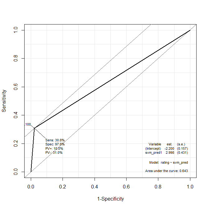

-> AUC : 0.643

 

 

2. 다수의 데이터셋에 SVM 모델 적용

- 만들어 놓은 20개의 train, test set에 대하여 SVM 모델을 적용한다. 

accuracy<-c()

for (x in 1:20){
	svm_model<-svm(rating~.-quality, data=train[[x]], type="C-classification")
	svm_pred<-predict(svm_model, test[[x]])
	tab <- table(svm_pred,test[[x]][["rating"]])
	accuracy<-c(accuracy, sum(tab[1,1], tab[2,2]) / sum(tab))
}

mean(accuracy)

[1] 0.8866667

sd(accuracy)

[1] 0.007478038

-> 평균 정확도 : 0.8866667, 정확도의 표준편차 : 0.007478038

 

3. cost 값을 바꿔가면서 SVM 모델 적용

-> kernel 옵션도 바꿔가면서 적용해봐야한다.

-> tune.svm() 함수를 이용하여 최적의 파라미터를 구할 수 있다.

3-1. cost 값 1, 2, 5, 10, 20 

- cost 값을 1, 2, 5, 10, 20으로 돌아가면서 적용해본다. 

# 표준정확도, 표준편차 리스트
accuracy<-list()

# 분류 기준값
cost_list<-c(1, 2, 5, 10, 20) 

for(i in 1:5){
	acc_svm<-c()
	for (x in 1:20){
		svm_model<-svm(rating~.-quality, data=train[[x]], type="C-classification", cost=cost_list[i])
		svm_pred<-predict(svm_model, test[[x]])
		tab <- table(svm_pred,test[[x]][["rating"]])
		acc_svm<-c(acc_svm, sum(tab[1,1], tab[2,2]) / sum(tab))
}
    accuracy[[i]]<-c(mean(acc_svm), sd(acc_svm))
}

accuracy <- data.frame(Reduce(cbind, accuracy))
colnames(accuracy) <- c(1, 2, 5, 10, 20) 
rownames(accuracy) <- c('mean', 'sd')

accuracy

               1           2          5          10          20
mean 0.886666667 0.887500000 0.88729167 0.892291667 0.894687500
sd   0.007478038 0.009218355 0.01042543 0.009774037 0.008799334

-> cost값이 커질수록 평균 정확도가 높아지고 정확도의 표준편차는 낮아지는 것을 알 수 있다. 

-> cost값을 더 키워서 테스트해봐야겠다. 

 

3-2. cost 값 50, 100, 200, 350, 500

- cost 값을 50, 100, 200, 350, 500으로 돌아가면서 적용해본다. 

# 표준정확도, 표준편차 리스트
accuracy<-list()

# 분류 기준값
cost_list<-c(50, 100, 200, 350, 500) 

for(i in 1:5){
	acc_svm<-c()
	for (x in 1:20){
		svm_model<-svm(rating~.-quality, data=train[[x]], type="C-classification", cost=cost_list[i])
		svm_pred<-predict(svm_model, test[[x]])
		tab <- table(svm_pred,test[[x]][["rating"]])
		acc_svm<-c(acc_svm, sum(tab[1,1], tab[2,2]) / sum(tab))
}
    accuracy[[i]]<-c(mean(acc_svm), sd(acc_svm))
}

accuracy <- data.frame(Reduce(cbind, accuracy))
colnames(accuracy) <- c(50, 100, 200, 350, 500) 
rownames(accuracy) <- c('mean', 'sd')

accuracy

             50        100        200        350        500
mean 0.89541667 0.89135417 0.88656250 0.88385417 0.88062500
sd   0.01260192 0.01139636 0.01325351 0.01291127 0.01312578

-> 20~100 사이의 정확도가 높아보인다. 

-> 이 사이에서 좀 더 세밀하게 테스트해볼 필요가 있어보인다. 

 

3-3. cost 값 20~100

- 정확도가 높은 20~100사이의 cost값을 비교해본다. 

# 표준정확도, 표준편차 리스트
accuracy<-list()

# 분류 기준값
cost_list<-c(20,30, 40, 50, 60, 70, 80, 90, 100) 

for(i in 1:9){
	acc_svm<-c()
	for (x in 1:20){
		svm_model<-svm(rating~.-quality, data=train[[x]], type="C-classification", cost=cost_list[i])
		svm_pred<-predict(svm_model, test[[x]])
		tab <- table(svm_pred,test[[x]][["rating"]])
		acc_svm<-c(acc_svm, sum(tab[1,1], tab[2,2]) / sum(tab))
}
    accuracy[[i]]<-c(mean(acc_svm), sd(acc_svm))
}

accuracy <- data.frame(Reduce(cbind, accuracy))
colnames(accuracy) <- c(20,30, 40, 50, 60, 70, 80, 90, 100) 
rownames(accuracy) <- c('mean', 'sd')

accuracy

              20         30         40         50         60         70
mean 0.894687500 0.89562500 0.89520833 0.89541667 0.89312500 0.89145833
sd   0.008799334 0.01066374 0.01143289 0.01260192 0.01326428 0.01308744
             80         90        100
mean 0.89177083 0.89041667 0.89135417
sd   0.01194826 0.01188932 0.01139636

 

3-4. 신뢰구간 그래프

- 95% 신뢰구간 그래프를 그려본다. 

accuracy <- t(accuracy)
plot(1:9, accuracy[,1], pch = 16, type = 'o',
	ylim = c(0.8, 1.0),
	ylab = 'Mean & CI', xlab = 'Cost', axes = F)
axis(1, at = 1:9, lab = c("20", "30", "40", "50", "60", "70", "80", "90", "100") )
axis(2, ylim = c(0.7, 1))
arrows(1:9, accuracy[,1] - 1.96 * accuracy[,2],
	1:9, accuracy[,1] + 1.96 * accuracy[,2],
	code = 3, angle = 90, length = 0.05)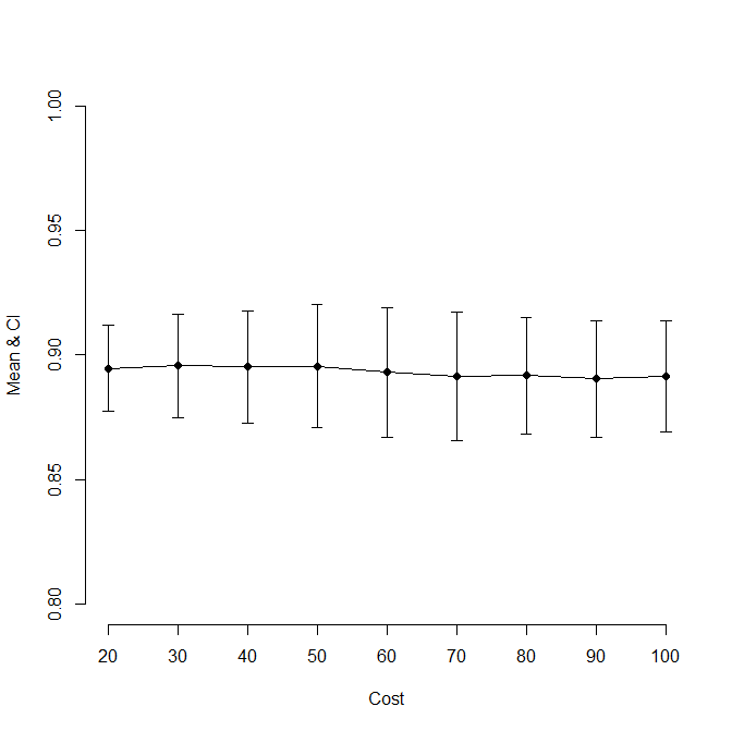

-> 표준 정확도가 거의 비슷해보이지만 신뢰구간의 크기가 꽤 차이가 있다. 

-> 따라서 신뢰구간이 가장 작은 20이 cost값으로 가장 적절하다고 생각한다.

-> 신뢰구간이 모두 겹치는 것을 보면 cost에 따라 큰 차이가 없다는 것을 알 수 있다. 

 

3-5. ROC curve

- cost 20에서의 ROC curve를 그려본다. 

svm_model<-svm(rating~.-quality, data=train[[1]], type="C-classification", cost=20)
svm_pred<-predict(svm_model, test[[1]])

svm_roc<-ROC(form=rating~svm_pred, data=test[[1]], plot="ROC")

-> AUC : 0.748

-> 처음에 cost값이 1이었을때와 비교하면 AUC, 민감도, 특이도 모두 증가하였다는 것을 알 수 있다. 

 

4. 모델 비교

- 그 동안 적용해 봤던 logistic regression과 decission tree를 svm과 비교한다. 

 

- logistic regression : 분류 기준값이 0.6일 때

- decission tree : 최소 가지치기 데이터수가 100개일 때

- svm : cost값이 20일 때

-> 그래프 그릴 때는 범위 맞춰주기

-> 가설 검정 해보기

 

library(ROCR)

4-1. ROC curve 비교

logit_model<-glm(rating ~ .-quality-citric.acid-residual.sugar-density-pH, data = train[[1]], family=binomial(link=logit))
tree_model<-rpart(rating~., data=train_dt[[1]], control=rpart.control(minsplit=threshold[100]))
svm_model<-svm(rating~.-quality, data=train[[1]], type="C-classification", cost=20)

logit_pred<-(predict(logit_model, test[[1]], type="response") >= 0.6)
tree_pred<-predict(tree_model, newdata=test_dt[[1]], type="class")
svm_pred<-predict(svm_model, test[[1]])

logit_pred<-prediction(as.numeric(logit_pred), test[[1]]$rating)
tree_pred<-prediction(as.numeric(tree_pred), test[[1]]$rating)
svm_pred<-prediction(as.numeric(svm_pred), test[[1]]$rating)

logit_pf<-performance(logit_pred, "tpr", "fpr")
tree_pf<-performance(tree_pred, "tpr", "fpr")
svm_pf<-performance(svm_pred, "tpr", "fpr")

plot(logit_pf,col="red")
par(new=TRUE)
plot(tree_pf,col="blue")
par(new=TRUE)
plot(svm_pf, col="green")
abline(a=0,b=1)

->  logistic regression : red, decission tree : blue, svm : green

-> svm, logistic regression, decission tree 순으로 그래프가 그려진다. 

-> svm 모델이 가장 적합하다고 평가할 수 있다.

 

4-2. Lift 비교

par(mfrow=c(1,3))

logit_lift <- performance(logit_pred, "lift","rpp")
plot(logit_lift, col ="red")
abline(v=0.2)

tree_lift <- performance(tree_pred, "lift","rpp")
plot(tree_lift, col ="blue")
abline(v=0.2)

svm_lift <- performance(svm_pred, "lift","rpp")
plot(svm_lift, col ="green")
abline(v=0.2)

-> svm 모델의 경우 상위 20% 집단에 대해서 랜덤 모델과 비교할 때 약 4배 이상의 성과 향상을 보이는 것을 확인할 수 있다. 

---

ref.

- R, SAS, MS-SQL을 활용한 데이터마이닝, 이정진

- [R을 활용한 머신러닝 06-1] 서포트 벡터 머신 Support Vector Machine 예제 / 실습 : 네이버 블로그 (naver.com)

- [ADP] R을 활용한 모형평가 방법(2) - Confusion matrix, ROC Curve, Gain chart (tistory.com)

- [R] 신용분석:예측적분석(서포트 벡터 머신을 이용한 모델링 | by 미완성의 신 | Medium