
티스토리 뷰
데이터 설명
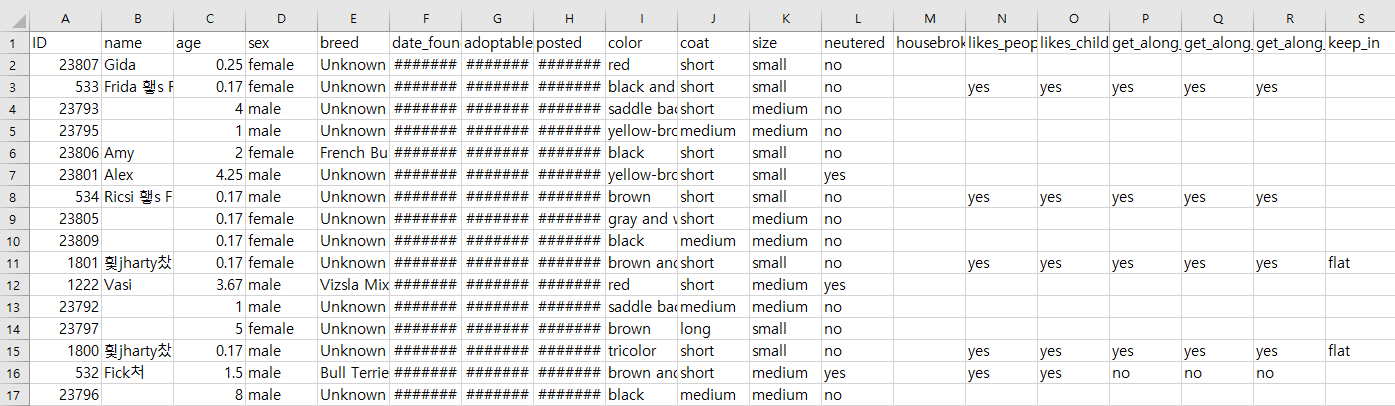
이름 : Adoptable Dogs
- 2019년 12월 12일 헝가리의 동물 보호소 데이터베이스의 2,937마리의 개에 대한 데이터이다.
데이터 불러오기
dogs<-read.csv("ShelterDogs.csv", header=T)
str(dogs)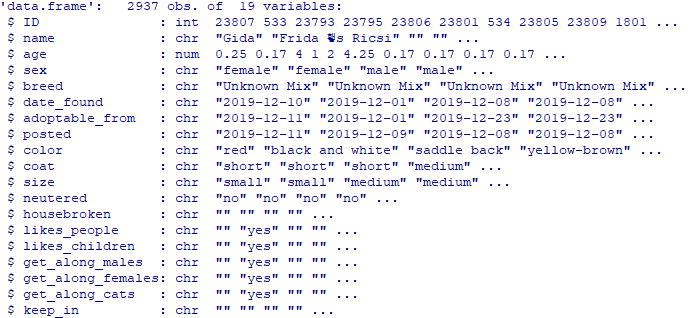
ID, name, age, sex 등 19개의 변수를 가지며, 총 2,937개의 데이터를 포함하고 있다.
데이터 분석
- 질적 데이터 분석 / 양적 데이터 분석
- 참고 : '[빅데이터/R] 데이터 분석해보기 1 - Adoptable Dogs' 수정하기 (tistory.com)
범주형 데이터 확보 및 연속형 데이터 이산형화(Discretization)
- 범주형 데이터 sex, coat, size, neutered와 연속형 데이터 age 총 5개의 변수를 사용하려 한다.
- 범주형 데이터의 경우 그 형태로 불러오면 되지만 연속형 데이터의 경우 범주형 데이터로 이산형화해주어야한다.
cust_dogs<-data.frame(dogs$sex, dogs$coat, dogs$size, dogs$neutered, dogs$age, stringsAsFactors = F)sapply(cust_dogs, class)
- 사용하기 편하게 이름을 변경해준다.
cust_dogs<-setNames(cust_dogs, c("sex", "coat", "size", "neutered", "age"))
- sex, coat, size, neutered 변수의 form을 character에서 factor로 변경시켜준다.
cust_dogs<-transform(cust_dogs, sex = as.factor(sex), coat = as.factor(coat), size = as.factor(size), neutered = as.factor(neutered))
- age 변수를 이산형화 한 age_cd 변수를 새로 만들어 준다.
나이가 0살-20살 까지 존재하므로 나이를 1-5, 6-10, 11-15, 16-20, 4가지의 범주로 나눌 수 있다.
cust_dogs<-within(cust_dogs, {
 age_cd = character(0)
 age_cd[age >= 0 & age <= 5] = "age_0_5"
 age_cd[age >= 6 & age <= 10] = "age_6_10"
 age_cd[age >= 11 & age <= 15] = "age_11_15"
 age_cd[age >= 16 & age <= 20] = "age_16_20"
 age_cd = factor(age_cd, level = c("age_0_5", "age_6_10", "age_11_15", "age_16_20"))
 })
head(cust_dogs)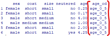
- 필요 없는 age 변수를 제거해준다.
cust_dogs_ar<-subset(cust_dogs, select = -c(age))str(cust_dogs_ar)
트랜잭션 데이터로 변환하기
- 연관 분석을 적용하기 위해 기존 범주형 데이터를 트랜잭션 데이터로 변환해준다.
library(arules)cust_dogs_ar_tr<-as(cust_dogs_ar, "transactions")cust_dogs_ar_tr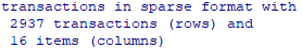
2937개의 트랜잭션과 16개의 항목이 생성되었다.
str(cust_dogs_ar_tr)
트랜잭션 데이터 보기
- 상위 3개의 트랜잭션 데이터를 출력하여 값을 확인하였다.
inspect(head(cust_dogs_ar_tr, 3))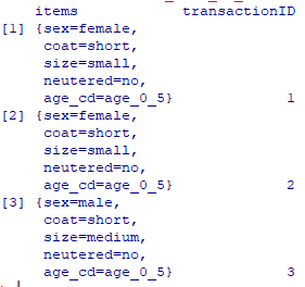
Apriori 알고리즘으로 연관규칙 생성하기
1-1. 최소 지지도(Support)와 최소 신뢰도(Confidence) 선택하기
- 각각 {0.1, 0.05, 0.01, 0.005}의 지지도와 {0.9, 0.8, 0.7, 0.6, 0.5, 0.4, 0.3, 0.2, 0.1}의 신뢰도에 대한 모든 규칙의 개수를 저장한다.
# Support and confidence values
supportLevels <- c(0.1, 0.05, 0.01, 0.005)
confidenceLevels <- c(0.9, 0.8, 0.7, 0.6, 0.5, 0.4, 0.3, 0.2, 0.1)

# Empty integers
rules_sup10 <- integer(length=9)
rules_sup5 <- integer(length=9)
rules_sup1 <- integer(length=9)
rules_sup0.5 <- integer(length=9)

# Apriori algorithm with a support level of 10%
for (i in 1:length(confidenceLevels)) {

  rules_sup10[i] <- length(apriori(cust_dogs_ar_tr, parameter=list(sup=supportLevels[1],
                                   conf=confidenceLevels[i], target="rules")))

}

# Apriori algorithm with a support level of 5%
for (i in 1:length(confidenceLevels)){

  rules_sup5[i] <- length(apriori(cust_dogs_ar_tr, parameter=list(sup=supportLevels[2],
                                  conf=confidenceLevels[i], target="rules")))

}

# Apriori algorithm with a support level of 1%
for (i in 1:length(confidenceLevels)){

  rules_sup1[i] <- length(apriori(cust_dogs_ar_tr, parameter=list(sup=supportLevels[3],
                                  conf=confidenceLevels[i], target="rules")))

}

# Apriori algorithm with a support level of 0.5%
for (i in 1:length(confidenceLevels)){

  rules_sup0.5[i] <- length(apriori(cust_dogs_ar_tr, parameter=list(sup=supportLevels[4],
                                    conf=confidenceLevels[i], target="rules")))

}
- 규칙의 개수를 보여주는 plot을 살펴본다.
library(ggplot2)
library(gridExtra)
# Number of rules found with a support level of 10%
plot1 <- qplot(confidenceLevels, rules_sup10, geom=c("point", "line"),
xlab="Confidence level", ylab="Number of rules found",
main="Apriori with a support level of 10%") +
theme_bw()
# Number of rules found with a support level of 5%
plot2 <- qplot(confidenceLevels, rules_sup5, geom=c("point", "line"),
xlab="Confidence level", ylab="Number of rules found",
main="Apriori with a support level of 5%") +
scale_y_continuous(breaks=seq(0, 10, 2)) +
theme_bw()
# Number of rules found with a support level of 1%
plot3 <- qplot(confidenceLevels, rules_sup1, geom=c("point", "line"),
xlab="Confidence level", ylab="Number of rules found",
main="Apriori with a support level of 1%") +
scale_y_continuous(breaks=seq(0, 50, 10)) +
theme_bw()
# Number of rules found with a support level of 0.5%
plot4 <- qplot(confidenceLevels, rules_sup0.5, geom=c("point", "line"),
xlab="Confidence level", ylab="Number of rules found",
main="Apriori with a support level of 0.5%") +
scale_y_continuous(breaks=seq(0, 130, 20)) +
theme_bw()
# Subplot
grid.arrange(plot1, plot2, plot3, plot4, ncol=2)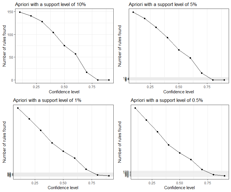
- 위와 같은 네개의 그래프를 색상으로 구분하여 하나의 그래프로 나타낼 수 있다.
# Data frame
num_rules <- data.frame(rules_sup10, rules_sup5, rules_sup1, rules_sup0.5, confidenceLevels)

# Number of rules found with a support level of 10%, 5%, 1% and 0.5%
ggplot(data=num_rules, aes(x=confidenceLevels)) +

  # Plot line and points (support level of 10%)
  geom_line(aes(y=rules_sup10, colour="Support level of 10%")) +
  geom_point(aes(y=rules_sup10, colour="Support level of 10%")) +

  # Plot line and points (support level of 5%)
  geom_line(aes(y=rules_sup5, colour="Support level of 5%")) +
  geom_point(aes(y=rules_sup5, colour="Support level of 5%")) +

  # Plot line and points (support level of 1%)
  geom_line(aes(y=rules_sup1, colour="Support level of 1%")) +
  geom_point(aes(y=rules_sup1, colour="Support level of 1%")) +

  # Plot line and points (support level of 0.5%)
  geom_line(aes(y=rules_sup0.5, colour="Support level of 0.5%")) +
  geom_point(aes(y=rules_sup0.5, colour="Support level of 0.5%")) +

  # Labs and theme
  labs(x="Confidence levels", y="Number of rules found",
       title="Apriori algorithm with different support levels") +
  theme_bw() +
  theme(legend.title=element_blank())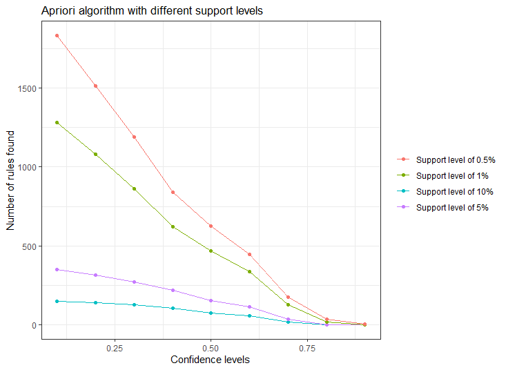
생각보다 많은 수의 규칙들이 생성되는 모습을 볼 수 있다. 따라서 더 큰 지지도를 가지고 다시 알아보려한다.
지지도와 신뢰도를 어떻게 선택해야하는 것인지 잘 모르겠다.
1-2. 최소 지지도, 최소 신뢰도 다시 찾아보기
- 이번에는 0.05 이상의 범주에서 지지도를 찾으려고한다.
- 각각 {0.5, 0.3, 0.1, 0.75}의 지지도와 {0.9, 0.8, 0.7, 0.6, 0.5, 0.4, 0.3, 0.2, 0.1}의 신뢰도에 대한 모든 규칙의 개수를 저장한다.
# Support and confidence values
supportLevels <- c(0.5, 0.3, 0.1, 0.075)
confidenceLevels <- c(0.9, 0.8, 0.7, 0.6, 0.5, 0.4, 0.3, 0.2, 0.1)

# Empty integers
rules_sup10 <- integer(length=9)
rules_sup5 <- integer(length=9)
rules_sup1 <- integer(length=9)
rules_sup0.5 <- integer(length=9)

# Apriori algorithm with a support level of 10%
for (i in 1:length(confidenceLevels)) {

  rules_sup10[i] <- length(apriori(cust_dogs_ar_tr, parameter=list(sup=supportLevels[1],
                                   conf=confidenceLevels[i], target="rules")))

}

# Apriori algorithm with a support level of 5%
for (i in 1:length(confidenceLevels)){

  rules_sup5[i] <- length(apriori(cust_dogs_ar_tr, parameter=list(sup=supportLevels[2],
                                  conf=confidenceLevels[i], target="rules")))

}

# Apriori algorithm with a support level of 1%
for (i in 1:length(confidenceLevels)){

  rules_sup1[i] <- length(apriori(cust_dogs_ar_tr, parameter=list(sup=supportLevels[3],
                                  conf=confidenceLevels[i], target="rules")))

}

# Apriori algorithm with a support level of 0.5%
for (i in 1:length(confidenceLevels)){

  rules_sup0.5[i] <- length(apriori(cust_dogs_ar_tr, parameter=list(sup=supportLevels[4],
                                    conf=confidenceLevels[i], target="rules")))

}
# Data frame
num_rules <- data.frame(rules_sup10, rules_sup5, rules_sup1, rules_sup0.5, confidenceLevels)
# Number of rules found with a support level of 10%, 5%, 1% and 0.5%
ggplot(data=num_rules, aes(x=confidenceLevels)) +
# Plot line and points (support level of 50%)
geom_line(aes(y=rules_sup10, colour="Support level of 50%")) +
geom_point(aes(y=rules_sup10, colour="Support level of 50%")) +
# Plot line and points (support level of 30%)
geom_line(aes(y=rules_sup5, colour="Support level of 30%")) +
geom_point(aes(y=rules_sup5, colour="Support level of 30%")) +
# Plot line and points (support level of 10%)
geom_line(aes(y=rules_sup1, colour="Support level of 10%")) +
geom_point(aes(y=rules_sup1, colour="Support level of 10%")) +
# Plot line and points (support level of 7.5%)
geom_line(aes(y=rules_sup0.5, colour="Support level of 7.5%")) +
geom_point(aes(y=rules_sup0.5, colour="Support level of 7.5%")) +
# Labs and theme
labs(x="Confidence levels", y="Number of rules found",
title="Apriori algorithm with different support levels") +
theme_bw() +
theme(legend.title=element_blank())
지지도 50%, 30%의 경우 생성되는 규칙이 매우 적으며, 반대로 지지도 7.5%의 경우 생성되는 규칙이 많기때문에, 우리는 지지도 10%를 선택 할 것이며, 최소 50%의 신뢰도를 선택하려한다.
2. 연관 규칙 생성하기
- apriori 알고리즘으로 최소 지지도 10%(0.1), 최소 신뢰도 50%(0.05) 이상인 연관 규칙들을 생성한다.
rules_sup10_conf50 <- apriori(cust_dogs_ar_tr, parameter=list(sup=supportLevels[3], conf=confidenceLevels[5], target="rules"))
- 지지도에 대한 내림차순으로 정렬 할 수 있다.
inspect(sort(rules_sup10_conf50))
동물 보호소의 중간 크기 강아지의 67%가 짧은 털을 가지고 있음을 알 수 있으며,
6살에서 10살인 강아지의 71%가 중간 크기의 몸집을 가지고 있음을 알 수 있다.
또한 성별이 남성이고, 중간 크기인 강아지의 62%가 짧은 털을 가지고 있음을 알 수 있다.
- 리프트(Lift) 기준으로 상위 5개의 규칙들을 살펴볼 수 있다.
inspect(head(sort(rules_sup10_conf50,by="lift"),5))
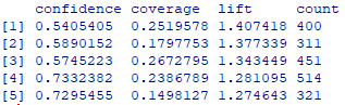
동물 보호소의 짧은 털을 가지며, 중간 크기이고 중성화를 한 강아지의 58%가 성별이 여성임을 알 수 있으며,
짧은 털을 가지며, 중성화를 한 강아지의 57%가 성별이 여성임을 알 수 있다.
또한 중성화를 하지 않은 강아지의 73%가 성별이 남성임을 알 수 있다.
3. 연관 규칙 시각화하기
library(arulesViz)plot(rules_sup10_conf50, measure=c("support", "lift"), shading="confidence")
plot(rules_sup10_conf50, method="graph")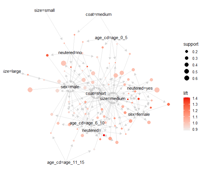
plot(rules_sup10_conf50, method="graph", control=list(layout=igraph::in_circle()))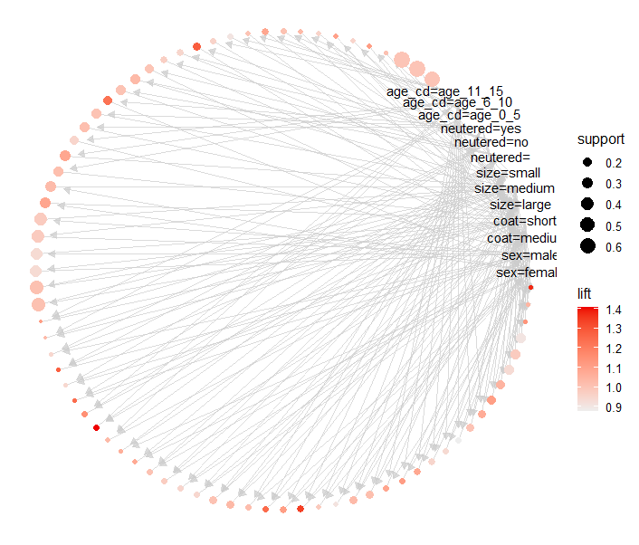
- Grouped Plot
plot(rules_sup10_conf50, method="grouped")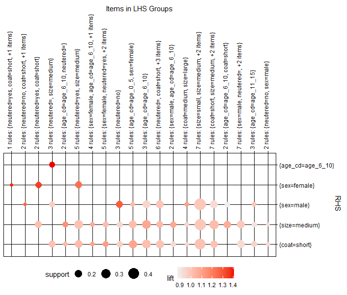
원의 크기가 지지도, 색이 향상도를 나타낸다.
- Paracoord Plot
plot(rules_sup10_conf50, method="paracoord")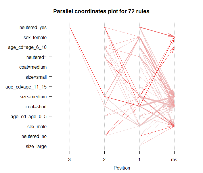
색의 진하기는 support를 나타내며, 그래프의 각 선이 꺾이는 곳을 기준으로 해석을 한다.
즉, "중성화를 했으며, 중간 크기이고, 털이 짧은 강아지는 성별이 여성이다." 라고 해석할 수 있다.
- Interactive Graph Plot
plot(rules_sup10_conf50, method="graph", interactive=T)

마우스를 가져다대면 반응하며, 원들을 마우스로 움직이며 관찰 할 수 있다.
Ref.
R, Python 분석과 프로그래밍의 친구 (by R Friend) :: '연속형 데이터의 연관규칙 분석' 태그의 글 목록 (tistory.com)
[R] 연관성 분석 : 네이버 블로그 (naver.com)
'Data > R' 카테고리의 다른 글
| [데이터 분석해보기] Bayes Classification (베이즈 분류) (feat. Mushroom) (1) | 2021.07.07 |
|---|---|
| [빅데이터] 분류분석 (Classification Analysis) (0) | 2021.07.07 |
| Linear Regression (선형 회귀) (0) | 2021.07.06 |
| 연관분석 (Association Analysis) (1) | 2021.07.05 |
| [데이터 분석해보기] Adoptable Dogs (0) | 2021.07.01 |